Regression Analysis is a technique to forecast the relationship between data variables of entities such as customers, orders, transactions, etc. These are the parameters based on which business decisions can be taken for sales, finance, and marketing operations. To understand this in a simpler way, let us take some examples.
Example 1 – Risk Analytics in Retail Banking
Credit risk scores of customers are built by the banking industry to predict the customer’s delinquency behavior and to evaluate the creditworthiness of each customer while processing loan applications.
Example 2 – Marketing Analytics in eCommerce
To predict customers’ buying patterns based on the customer’s past transactions from an online portal. The e-commerce industry is highly competitive so they use analytics to predict customers’ purchasing patterns.
Example 3 – Pricing Analytics in Stock Market
Stockbrokers and investors use analytics to forecast stock pricing based on the past 52-week pricing trend and many other parameters. The analytics helps them to make the decisions on buying or selling the stocks based on the future pricing predictions.
Example 4 – Behavioral Analytics in Human Resource Industry
Human resource departments/companies use analytics to predict employees’ behavioral patterns that will enable them to decide the increment or promotion to be given on a yearly basis.
Regression Analysis Basics
Before we go for how to do regression in Excel by taking a case study, let us understand the dataset and its components.
Population vs. Sample
The population is referred to as all members of a defined group that are considered for studying information on data-driven decisions. For example – The current inflation rates of EU countries.
A sample is a part of the “population”. It can be biased or unbiased. For example – The current inflation rates of EU countries having per capita income < 50000 EURO per annum.
Types of Data Variables
The below diagram shows the types of data variables under each category.

Data Snapshot
The table below gives an example of a data snapshot with different data variables.
| # | Cust.Name | Cust. ID | No.Of credit cards | Gender | Marital status | Age | Annua lSalary | Monthly Credit Card Usage |
| 1 | Josh | 111669 | 5 | F | Never Married | 43 | 88,001 | Low |
| 2 | John | 223112 | 6 | M | Married | 24 | 592,330 | Low |
| 3 | Alen | 189123 | 4 | M | Divorced | 50 | 272,304 | Low |
| 4 | Chaya | 171690 | 3 | F | Married | 37 | 140,400 | Low |
| 5 | Dandre | 16625 | 6 | M | Never Married | 23 | 105, 234 | Low |
| 6 | Justin | 149171 | 7 | M | Divorced | 34 | 358,534 | Low |
| 7 | Neil | 169254 | 5 | M | Married | 36 | 510,321 | Low |
| 8 | Emily | 149771 | 2 | F | Never Married | 26 | 164,732 | Low |
| 9 | Janice | 175646 | 2 | F | Married | 35 | 103,345 | Low |
| 10 | Farhan | 170639 | 4 | M | Never Married | 63 | 724,788 | Low |
| 11 | Tony | 113136 | 3 | M | Married | 70 | 105,450 | Low |
Let us understand the data variables available in the above table.
| # | Cust.Name | Cust. ID | No.of credit cards | Gender | Marital Status | Age | Annual Salary | Monthly Credit Card Usage |
| – | – | – | Numerical (Discrete) | Categorical (Binary) | Categorical (Nominal) | Numerical (Discrete) | Numerical (Continuous) | Categorical (Ordinal) |
Summarizing Data
The next step is to summarize data in a presentable format that will give the report on which analysis can be done. The ways to summarize the data are as follows:
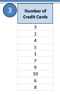
- Frequency Distribution – this is a simple way of counting distinct discrete values. For example – The number of credit cards owned by 3000 customers as sample data. Can be shown in tabular format or as a graph using Excel.

Steps to do this in Excel:
- Go to the Data tab in your Excel Worksheet.

- Click Advanced. The dialog is shown

- Go to the Number of Cards column. Sort them into ascending order of values.
- Insert the formula in # of customers to set the frequency.
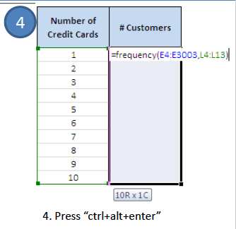
- You will get the values below.

- Go to the Insert tab. Click the Column icon. Select the 2-D Chart.

- The chart will be generated and shown below.

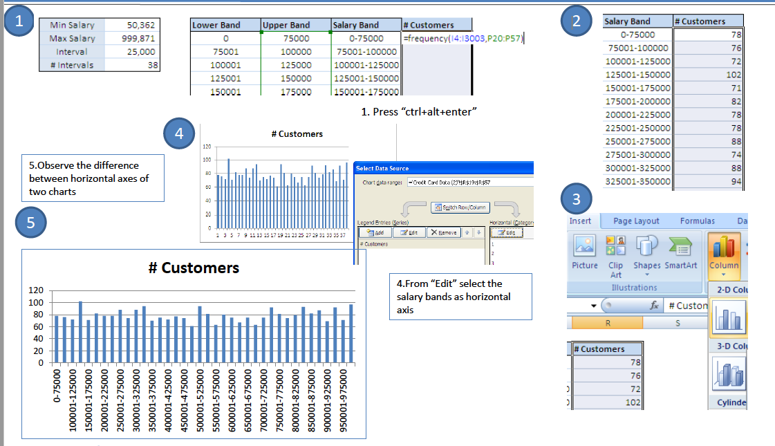
- Grouped Frequency Distribution – this is a method to summarize discrete variables having a large number of observations and a range of values. For example – The number of customers falling under different salary ranges or groups.

Follow the steps in Excel as per the instructions given on the screen below.
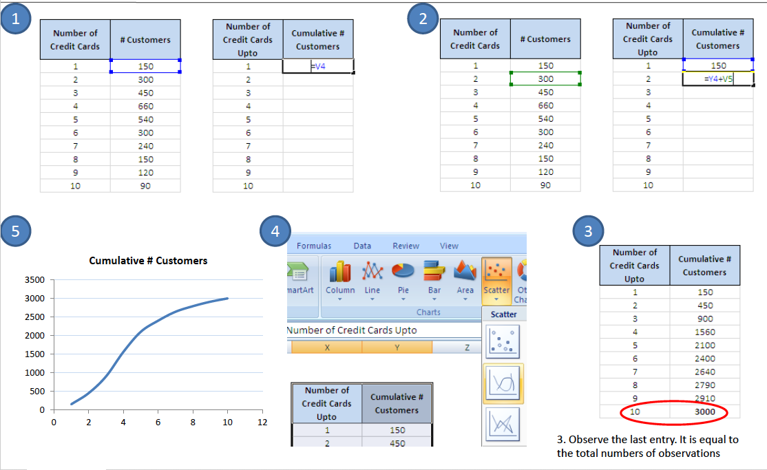
- Cumulative Frequency Distribution – this is obtained by accumulating the frequencies to give the total number of observations up to and including the value or group in question. Illustration as per the screen below.
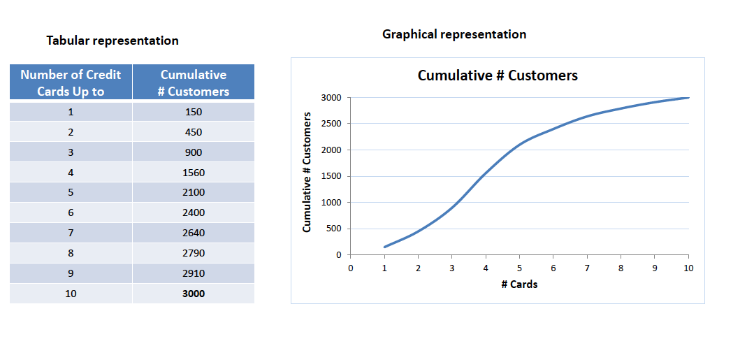
Steps to calculate the cumulative frequency distribution are given on the screen below.
- Stem Leaf Diagram – this technique is used in a limited set of data. For a large set of data, this method is not used. Example: Given the age of 20 individuals in years.

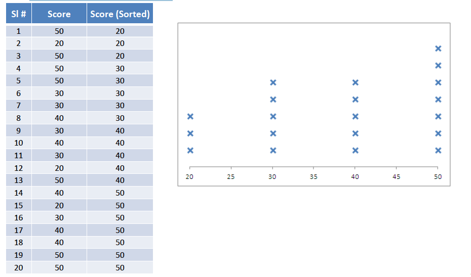
- Line Plots – this technique is also not suitable for a large set of data. It is not extensively used in the industry. Example: Given test scores of 20 students.
The measure of Central Tendency – Median
The central tendency measure is robust to the effects of extreme observations.
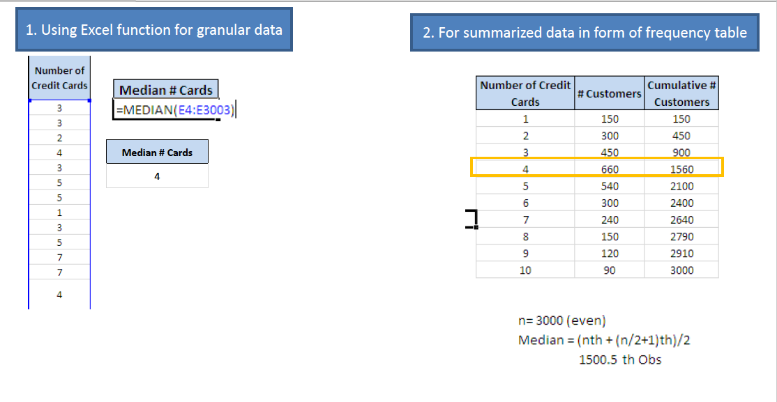
The median is a value, which splits the data set into two equal halves. Example – Calculate the median for a sample of 3000 individuals having credit cards along with a demonstration of extreme observations.
The measure of Central Tendency – Mode
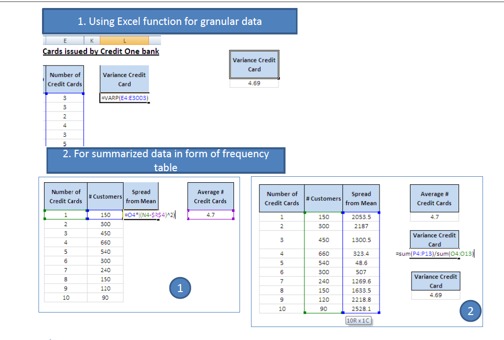
It is the value that occurs with the greatest frequency or the most typical value. For Example, finding the mode for a sample of 3000 individuals having credit cards. Excel has an in-built function “Mode” for granular data. For summarized data, it can be found easily by visual inspection. Illustration as below.

Measure of Spread
The different measures of spread are –
- Variance and Standard Deviation – below screen shows how to calculate the values.
- The Range – It is a very simple measure of spread defined, as its name suggests, by the difference between the largest and smallest observations in the data set.

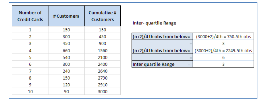
- The Interquartile range – the quartiles divide a set of data into four quarters. They are denoted by Q1, Q2, and Q3. Q1 is called the lower quartile and Q3 is the upper quartile. The following image shows how to calculate the Interquartile Range for a sample of 3000 individuals having credit cards.
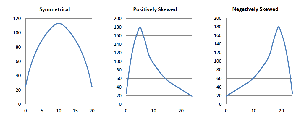
Symmetry and Skewness of data
It represents the shape of the distribution of a dataset, that is, whether it is symmetric or skewed to one side or the other. The approximate shape of a distribution can be determined by looking at a histogram. The below diagram shows the mean, median, mode, and variance for symmetric and skewed data.
A tabular representation of data is shown below.

After evaluating the dataset by the above measures and techniques, a regression analysis can be conducted. Now, the question is which type of regression model is required for predictions.
The next section describes the measures that will state the relationship between the data variables and determine how strong the relationship is between identified variables.
Regression Analysis Models
The following are different techniques or formulas that are used to do regression analysis. These techniques are nothing but different formulas or equations that are used to determine the relationship between X and Y variables.
Covariance and correlation coefficient are the measures used in regression analysis.
- Covariance is a measure that helps to find out the direction of the relationship between the x variable and y variables. In simple terms, what happens to y when x increases or decreases.
The following equation is used to determine the covariance measure.

- A correlation coefficient is a measure that tells how strong the linear relationship is between X and Y variables. It is termed an r-value that determines the quality of a model. The parameter is represented by p or r values.
- Population correlation is denoted by ρ (rho)
- Sample correlation is denoted by r.
The following equation is used to determine the correlation coefficient measure for population data.

In real-life data analytics, the correlation measure is calculated on sampling distribution. There are a couple of reasons why sampling is used for analytics.
Features of ρ and r
- The physical impossibility of checking all items in the population.
- The cost of studying all the items in a population.
- The sample results are usually adequate.
- Contacting the whole population would often be time-consuming.
- Unit free and ranges between -1 and 1
- The closer to -1, the stronger the negative linear relationship
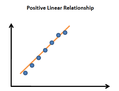
- The closer to 1, the stronger the positive linear relationship
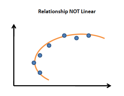
- The closer to 0, the weaker the linear relationship
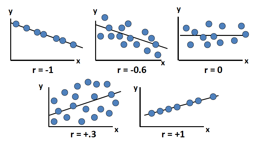
Negative Linear Relationship

Positive Linear Relationship
Relationship Not Linear
No Relationship

Tools used to do Regression Analysis
Following software tools are the most used in performing Regression Analysis. The oldest tool is Microsoft Excel.
- SAS (www.sas.com/)
- SPSS (http://www-01.ibm.com/software/analytics/spss/ )
- R (http://www.r-project.org/)
- Microsoft Excel (http://office.microsoft.com/en-in/)
As the spectrum of analytics is widened, dataset volume has increased, the data scientists have started using Python.
We will see a case study to run regression analysis in Excel.
Case Study
An Auto Insurance company has the data of “Loss” amount and policy-related information. The company wants to know the factors responsible for losses in a multivariate fashion using a regression model.
Prior to running the regression model, the following things need to be in place.
- Variable identification –
- Identifying the dependent (response) variable.
- Identifying the independent (explanatory) variables.
- Variable categorization (e.g. Numeric, Categorical, Discrete, Continuous, etc.)
- Creation of Data Dictionary
- Response variable exploration
- Distribution analysis
- Percentiles
- Variance
- Frequency distribution
- Outlier treatment
- Identify the outliers/threshold limit
- Cap/floor the values at the thresholds
- Distribution analysis
- Independent variable analyses
- Identify the prospective independent variables (that can explain the response variable)
- Bivariate analysis of response variable against independent variables
- Variable treatment /transformation
- Grouping of distinct values/levels
- Mathematical transformation e.g. logs, splines, etc.
After performing the above data-related activities, the last step is iterative in terms of running the regression.
Fitting the regression (first time)
- Check for correlation between independent variables
- This is to take care of Multicollinearity
- Variable selection
- Check for the most suitable transformed variable
- Select the transformation giving the best fit
- Reject the statistically insignificant variables
Fitting the regression (iteration)
- Analysis of results
- Model comparison
- Model performance check
- Actual vs Predicted comparison
Steps to do regression analysis in Excel
We will perform the following steps in Excel with reference to the case study explained in the section above.
Data Analysis
Step 1. Snapshot of Data and Data Description

The above data contains policy holders’ and loss amount information (variables)
- Policy Number
- Age
- Years of Driving Experience
- Number of Vehicles
- Gender
- Married
- Vehicle Age
- Fuel Type
- Losses (Dependent/Response Variable)
A Data Dictionary is formed as below.
| Sl # | Variable Name | Variable Description | Values Stored | Variable Type |
| 1 | Policy Number | Unique Policy Number | Unique value identifying the policy | Identifier |
| 2 | Age | Age of Policyholder | 16, 17,…,70 | Numerical (Discrete) |
| 3 | Years of Driving Experience | Years of Driving Experience of the Policyholder | 0,1,….,53 | Numerical (Discrete) |
| 4 | Number of Vehicles | Number of Vehicles insured under the policy | 1,2,3,4 | Numerical (Discrete) |
| 5 | Gender | Gender of the Policyholder | F, M | Categorical (Binary) |
| 6 | Married | Marital status of the Policyholder | Married, Single | Categorical (binary) |
| 7 | Vehicle Age | Age of vehicle insured under the policy | 0,1,…,15 | Numerical (Discrete) |
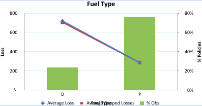
| 8 | Fuel Type | Fuel type of the vehicle insured | D, P | Categorical (Binary) |
| 9 | Losses | Loss amount claimed under the policy | Range: 13- 3500 | Numerical (Continuous) |
Step 2. Frequency Distribution – Loss amount

Step 3. Calculate Capped Losses using grouped frequency distribution

Step 3. Perform variable analysis in Excel. The first bivariate profiling we will do for Age vs. Capped Loss for policies.

Step 4. The second bivariate profiling we will do for Years of Driving Experience vs. Capped Loss for policies.

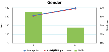
Step 5. The next bivariate profiling we will do for Gender vs. Capped Loss for policies.
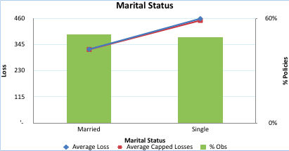
Step 6. The next bivariate profiling we will do for Marital Status vs. Capped Loss for policies.
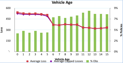
Step 7: The next bivariate profiling we will do for Vehicle Age vs. Capped Loss for policies.
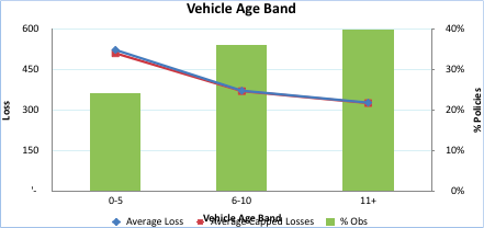
Step 8: The next bivariate profiling we will do for Vehicle Age Band vs. Capped Loss for policies.
Step 9: The next bivariate profiling we will do for Vehicles vs. Capped Loss for policies.

Step 10: The next bivariate profiling we will do for Fuel Type vs. Capped Loss for policies.
Preparing Excel for Regression Analysis
Step 1: Open the Office icon from the toolbar.

Step 2: Go to Excel Options.
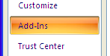
Step 3: Click Add-Ins.
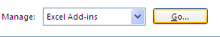
Step 4: From the Manage drop-down, select Excel Add-ins.
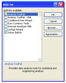
Step 5: Select the Analysis Toolpak check box and the Solver Add-in check box.
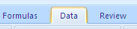
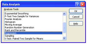
Step 6: Select the Data tab. Click Data Analysis.

Step 7: In the Data Analysis dialog box, click Regression.
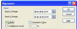
Step 8: Select the data cell reference range. Click OK.
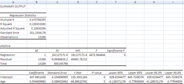
Step 9: See the summary results as below.
Step 10: Picking up the variables based on the following activities.
We will perform the following tests to select by running :
- Multicollinearity
- Banding of variables
- Statistical significance of variables tested
List of independent variables:
- Age
- Age Band
- Years of Driving Experience
- Number of Vehicles
- Gender
- Married
- Vehicle Age
- Vehicle Age Band
- Fuel Type
“Age” and “Years of Driving Experience” are highly correlated (Correlation Coefficient = 0.9972). We can use either of the variables in the regression.
Fit two separate models using either of the variables one at a time. Check for the goodness of fit (R2 in this case). The variable producing higher R2 gets accepted.
Age
| Regression Statistics (Age) | |
| Multiple R | 0.475766 |
| R Square | 0.226354 |
| Adjusted R Square | 0.226303 |
| Standard Error | 201.2306 |
| Observations | 15290 |
Years of Driving Experience
| Regression Statistics(Yrs Driving Experience) | |
| Multiple R | 0.475273 |
| R Square | 0.225885 |
| Adjusted R Square | 0.225834 |
| Standard Error | 201.2916 |
| Observations | 15290 |
- R2 for Age > R2 for Years of Driving Experience
- Reject Years of Driving Experience
Banding of Variables
- Investigate whether to use “Age” or “Age band”
- Fit regression independently using “Age” and “Age Band”
- Before fitting regression, “Age Band” needs to be converted to numerical form from categorical. Replace “Age Band” values with “Average Age” for the particular band.
| Age Band | Sum of Age | # Policies | Average Age |
| 16-25 | 93,770.0 | 4,563.0 | 20.6 |
| 26-59 | 270,793.0 | 6,384.0 | 42.4 |
| 60+ | 282,636.0 | 4,343.0 | 65.1 |
- Regressions results using “Age” and “Average Age”
| Regression Statistics (Age) | |
| Multiple R | 0.475766 |
| R Square | 0.226354 |
| Adjusted R Square | 0.226303 |
| Standard Error | 201.2306 |
| Observations | 15290 |
| Regression Statistics (Average Age) | |
| Multiple R | 0.509969 |
| R Square | 0.260068 |
| Adjusted R Square | 0.26002 |
| Standard Error | 196.7971 |
| Observations | 15290 |
- R2 for Average Age > R2 for Age
- Select “Average Age”
Investigate whether to use “Vehicle Age” or “Vehicle Age band”
- Fit regression independently using “Vehicle Age” and “Vehicle Age Band”
- Before fitting regression, “Vehicle Age Band” needs to be converted to numerical form from categorical. Replace “Vehicle Age Band” values with “Vehicle Average Age” for the particular band.
| Vehicle Age Band | Sum of Vehicle Age | # Policies | Average Vehicle Age |
| 0-5 | 9,229 | 3,688 | 2.50 |
| 6-10 | 44,298 | 5,523 | 8.02 |
| 11+ | 78,819 | 6,079 | 12.97 |
- Regressions results using “Vehicle Age” and “Average Vehicle Age”
| Regression Statistics (Vehicle Age) | |
| Multiple R | 0.289431325 |
| R Square | 0.083770492 |
| Adjusted R Square | 0.083710561 |
| Standard Error | 218.9903277 |
| Observations | 15290 |
| Regression Statistics (Average Vehicle Age) | |
| Multiple R | 0.303099405 |
| R Square | 0.09186925 |
| Adjusted R Square | 0.091809848 |
| Standard Error | 218.0203272 |
| Observations | 15290 |
- R2 for Average Vehicle Age > R2 for Vehicle Age
- Select “Average Vehicle Age”
Now, we have identified the variables that can be used in fitting the regression model.
- Age Band in the form of “Average Age” of the band (selected out of “Age” and “Age Band”). Also got selected over “Years of Driving Experience”.
- Number of Vehicles
- Gender
- Married
- Vehicle Age Band in the form of “Average Vehicle Age” of the band (selected out of “Vehicle Age” and “Vehicle Age Band”).
- Fuel Type
Step 11: Categorical variables to be converted to their numerical equivalent (0,1)
- Gender (F = 0 and M = 1)
- Married (Married = 0 and Single = 1)
- Fuel Type (P = 0, D = 1)
Snapshot of the final data on which we will run the multivariate regression.

Step 11: Run Regression.
Summary of Output
| SUMMARY OUTPUT | ||||||||
| Regression Statistics | ||||||||
| Multiple R | 0.865972274 | |||||||
| R Square | 0.749907979 | |||||||
| Adjusted R Square | 0.749809794 | |||||||
| Standard Error | 114.4310136 | |||||||
| Observations | 15290 | |||||||
| ANOVA | ||||||||
| df | SS | MS | F | Significance F | ||||
| Regression | 6 | 600073213.5 | 100012202.3 | 7637.751088 | 0 | |||
| Residual | 15283 | 200122584.4 | 13094.45688 | |||||
| Total | 15289 | 800195798 | ||||||
| Coefficients | Standard Error | t Stat | P-value | Lower 95% | Upper 95% | Lower 95.0% | Upper 95.0% | |
| Intercept | 624.56529 | 5.29192 | 118.02233 | 0.00000 | 614.19249 | 634.93809 | 614.19249 | 634.93809 |
| Avg Age | -5.55974 | 0.06546 | -84.93889 | 0.00000 | -5.68804 | -5.43144 | -5.68804 | -5.43144 |
| Number of Vehicles | 0.17875 | 0.97039 | 0.18420 | 0.85386 | -1.72333 | 2.08082 | -1.72333 | 2.08082 |
| Gender Dummy | 50.88326 | 1.89081 | 26.91084 | 0.00000 | 47.17705 | 54.58947 | 47.17705 | 54.58947 |
| Married Dummy | 78.39837 | 1.92148 | 40.80106 | 0.00000 | 74.63204 | 82.16469 | 74.63204 | 82.16469 |
| Avg Vehicle Age | -15.14220 | 0.26734 | -56.63987 | 0.00000 | -15.66623 | -14.61818 | -15.66623 | -14.61818 |
| Fuel Type Dummy | 267.93559 | 2.74845 | 97.48614 | 0.00000 | 262.54830 | 273.32287 | 262.54830 | 273.32287 |
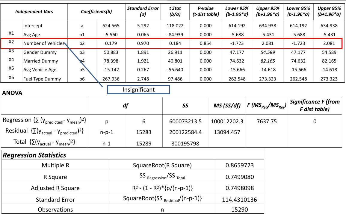
Results Interpretation
Significant Test

Significance test of coefficients based on Normal distribution
- H0: b is no different than 0 (i.e. 0 is the coefficient when the variable is not included in regression)
- H1: b is different than 0
Test statistic, Z = (b-0)/σ (at 95% two tailed confidence interval, Z = 1.96)
Confidence interval = (b – 1.96 * σ, b + 1.96 * σ)
For the variable to be significant, the interval must not contain “0”.
Example1: Avg Age.
Confidence interval = (-5.560-1.96*0.065, -5.560+1.96*0.065) = (-5.688, -5.431)
No zero in the interval. Hence, significant.
Example2: Number of Vehicles
Confidence interval = (0.179-1.96*0.970, 0.179+1.96*0.970) = (-1.723, 2.080)
Zero is present in the interval. Hence, insignificant.
Summary output after removing insignificant variables.
Predicted Losses = 625.004932715948 – 5.5596551344537 * Avg Age + 50.8828923910091 * Gender Dummy + 78.4016899779131 * Married Dummy -15.1420259903571 * Avg Vehicle Age + 267.935139741526 * Fuel Type Dummy
Interpretation
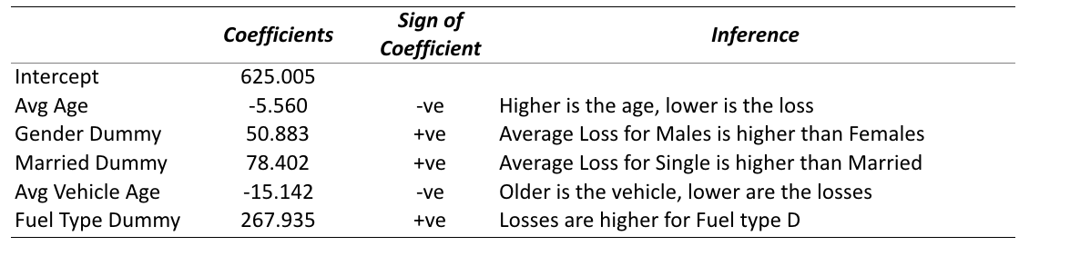
Takeaway
Running regression in Excel gives you more confidence in your model as you are running each step manually. It is a time-consuming and lengthy process, but you get to learn more about datasets and output summaries. Other tools such as R, SAS, and Python give you quick results but you will not be able to know the algorithm behind the code that is executed and has given you the results.
You may also like:
How to do Indent Text in Excel Sheet
How To Delete Multiple Rows in Excel Sheet at Once
How to Create a Waterfall Chart in Microsoft Excel?
