How to Use Google Sheets Unique Values Function?

Google Sheets’ unique function works as a query to return a set of unique values from the selected cell range (row(s) or column(s)). Putting the reference range in a column with a unique function will give you the results as expected.

The unique function is very useful when doing data analysis tasks. You may come across the use cases where you need to filter a dataset to remove duplicate records, identify the data with unique values of a property, and so on.

Some data examples are given below to explain how the unique formula works.

• To find out the unique score of the exam participants and their classrooms.
• To find out the unique price range of mobile sets based on their brands
• To find out the unique assignees of the tickets they are assigned, status, and type of tickets available
• To find out the number of goods received in a week

Example 1 – UNIQUE() function Google Sheets with 2 Columns

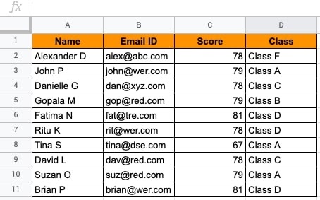
This dataset contains exam participants from different classrooms and their scores. We need to find out the unique scores from the classes they belong to.

Let us see how to use the UNIQUE() function to retrieve the values.

1. In a blank cell of the area in which you want the results to be populated.
2. Enter the function as shown in cell B13 as below.

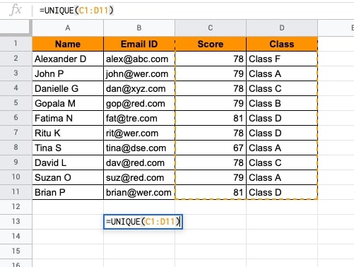
3. We have selected the column range C1:D11 to find out the unique values.
4. Press ENTER to get the results.

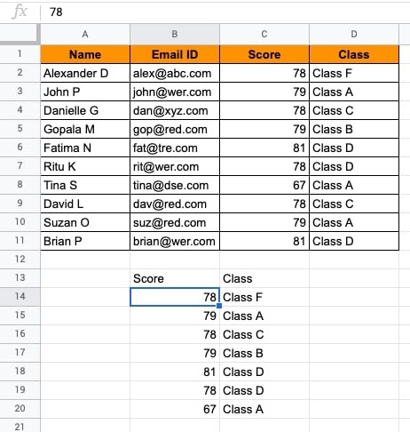
5. You will see that 7 rows are unique out of 11 rows. 
6. To further filter the unique score, you can put the UNIQUE() function for scores.
7. To do so, choose the reference range of the Score column.

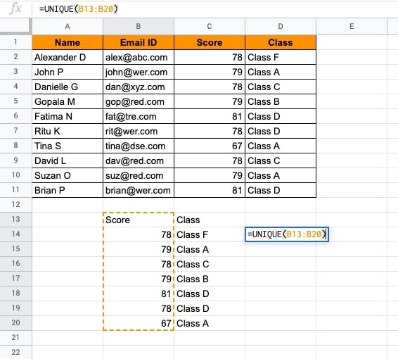
8. Put the function with reference cell range and ENTER.
9. The results are shown below.

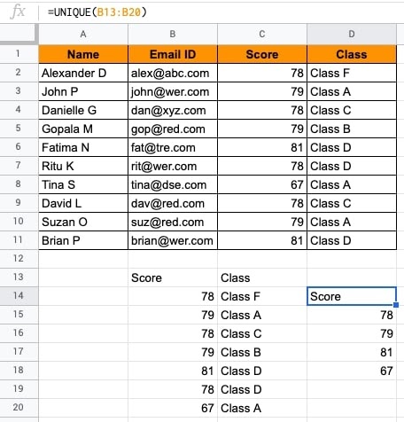
10. You have filtered unique values of the score (results are D14:D18).
11.  Further, the score results can be sorted in the ascending or descending order. Put the SORT() function by selecting the reference range of D14:D18.

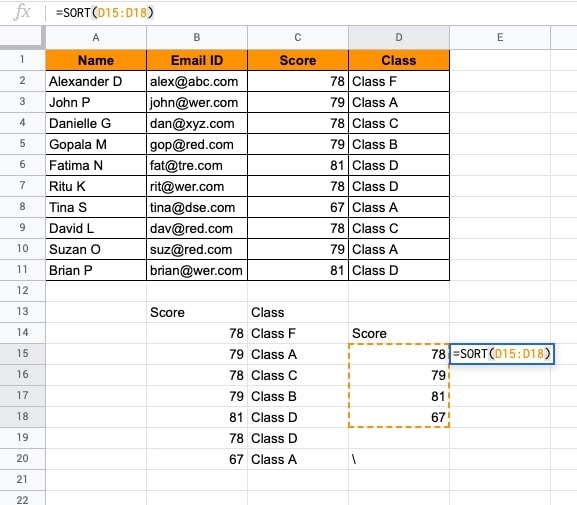
12. ENTER. The results will be sorted in the ascending order of value.

13. The results values are shown with MIN to MAX range once sorted.

The score analysis can be performed using the UNIQUE() and the SORT() functions.

Example 2 UNIQUE() function Google Sheets with TRANSPOSE()

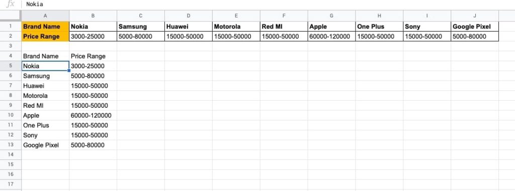
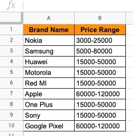
You have a dataset with row headers and values of mobile phone brands and their price range.

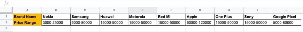
To perform analysis, it is recommended to convert the dataset to a vertical view. 

1. Use the TRANSPOSE() function to change it to a vertical view. 

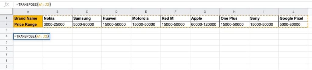
2. ENTER. You will see the data in a vertical view.

3. You can remove the horizontal view or move the transposed view to another sheet.
4. Put the UNIQUE() function on the Price Range column.

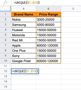
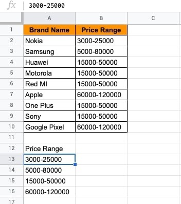
5. ENTER. The unique ranges will be shown.

Example 3 – UNIQUE() with a Single Column at a time

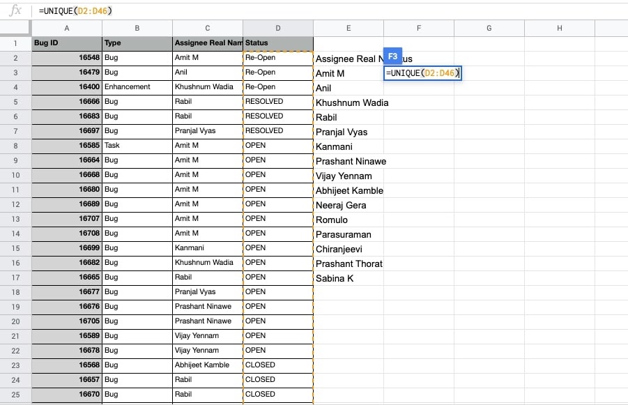
This dataset contains a list of tickets assigned to the helpdesk team with ticket IDs. We will find out the team members who will need to resolve the tickets. 

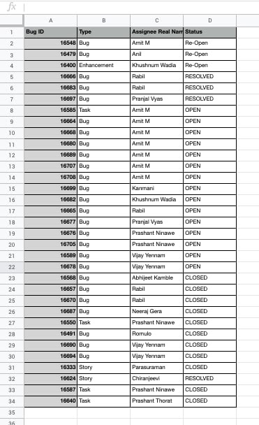
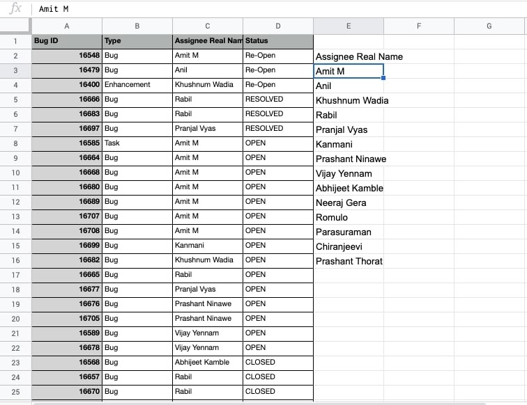
1. Choose the Assignee Real Name column while using the UNIQUE() function.

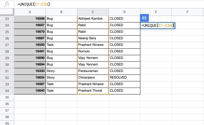
2. ENTER. You will see the unique team members that are assigned one or more tickets.

3. If the dataset is appended by more rows, you can simply refresh the results with updated values.

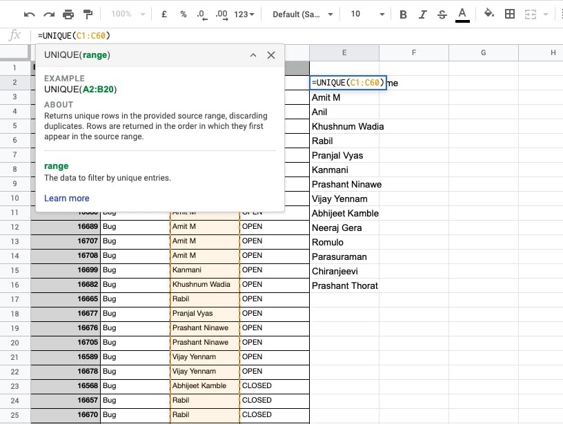
4. Increase the cell reference range and the results will be automatically updated.

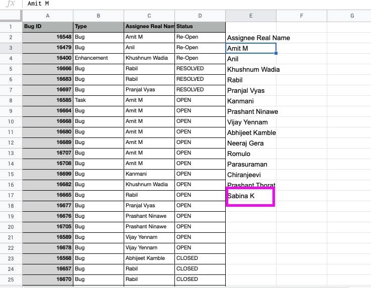
5. The results are shown with updated values.
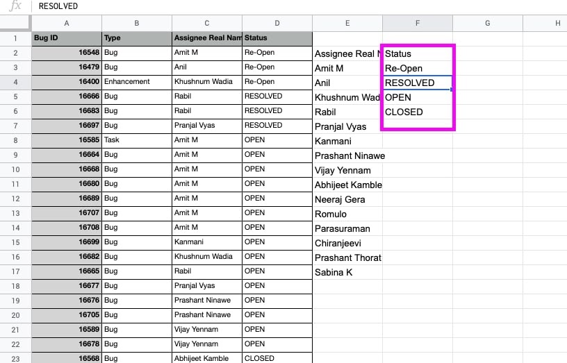
6. Similarly, you can identify the type of status(es) available in the dataset.
7. Put the UNIQUE() function in the blank cell and type the cell reference of the Status column inside the function.

8. ENTER. The unique values of status(es) will be shown.

9. Similarly, you can find out the type of tickets also can be filtered.

Example 4 UNIQUE() with COUNTIF() and SUMIF()

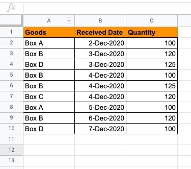
This dataset contains a list of goods received data wise. We will find out the count of each type of good received. This will result in retrieving a single good count. We will extend the function to retrieve the unique values returned for all goods.

1. To find the count of Box A received in the duration, we will put the formula below.

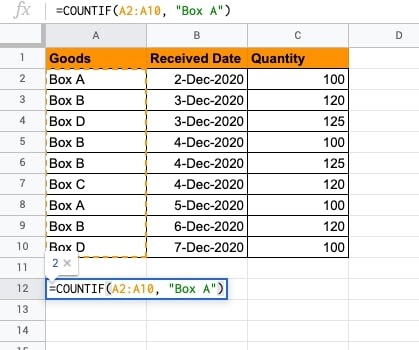
2. The results of Box A count come to 2. Further, we will see how to view the unique values of all goods received.
3. Combine the UNIQUE() and COUNTIF functions to retrieve the results as expected.

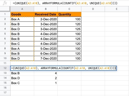
4. You will see the unique count of boxes received within the specified period.
5. It is that simple!

You can also retrieve SUM TOTAL of the quantity received per box using the UNIQUE() and SUMIF functions. 

1. First, find out the unique range of goods (boxes in this example.)
2. Then, use the SUMIF() function to specify the range of goods and their quantities.

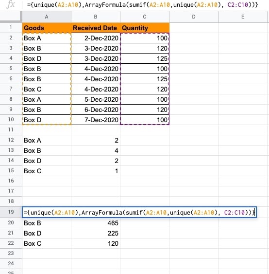
3. The UNIQUE() function identifies the goods to obtain the total quantity per box.
4. It’s quite useful.

Example – The COUNTUNIQUE() function

This dataset contains a range of values. To find out the count of unique values/price range, the COUNTUNIQUE() function is used.

1. To obtain the count of unique price ranges for the brands available, but the function as shown below.

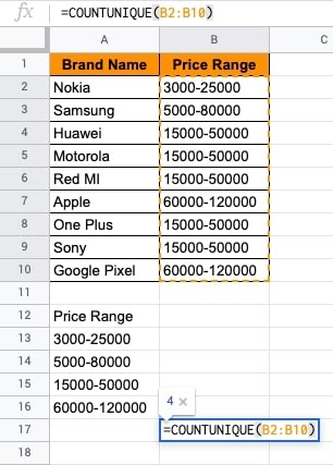
2. ENTER. You will see the 4 brands have a unique price range. The function returns the count of 4.
3. You can further evaluate the unique values that brands offer. After obtaining the subset of data, you can use it in multiple ways.

Takeaway

Google sheets are faster in performance and provide a range of financial functions to performing data analysis. Excel users find it so easy to use Google Sheets as all functions are similar. In addition to that, database experts also can easily use Google Sheets as it provides Query syntax that is very similar to writing query statements to retrieve results from the database tables.

The Google Sheets have captured all target segments for the usage – starting from a fresher to database expertise. 

You may also like:

• How to do Indent Text in Excel Sheet
• How To Delete Multiple Rows in Excel Sheet at Once
• How to Create a Waterfall Chart in Microsoft Excel